 Posted by
 Bayesian optimization (BO) is a sample-efficient optimization method focused on solving the problem
when the objective function f_0 is unknown or expensive to evaluate. At a high level, BO behaves just like a human learner: It iteratively updates its understanding of the environment based on historical information and automatically decides what to learn next.
This blog contains two parts: In Part 1, we introduce the basic idea of BO. In Part 2, we further examine BO by taking into account uncontrollable contextual information and constraints.
1. Making the Best Cake
Let us start with an example of cake making. Our goal is to find the right amount of ingredients that maximize our client’s satisfaction. We have no idea how client satisfaction relates to the amount of ingredients mathematically, so the classical gradient-based optimization methods cannot be used.
Moreover, it takes one hour to bake a cake and it is too costly to try all possibilities. Therefore, any methods requiring lots of function evaluations, such as grid search, random search, and most derivative-free optimization algorithms, are out of our consideration.
For simplicity, let us say that we only need to find out the perfect amount of sugar.
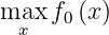
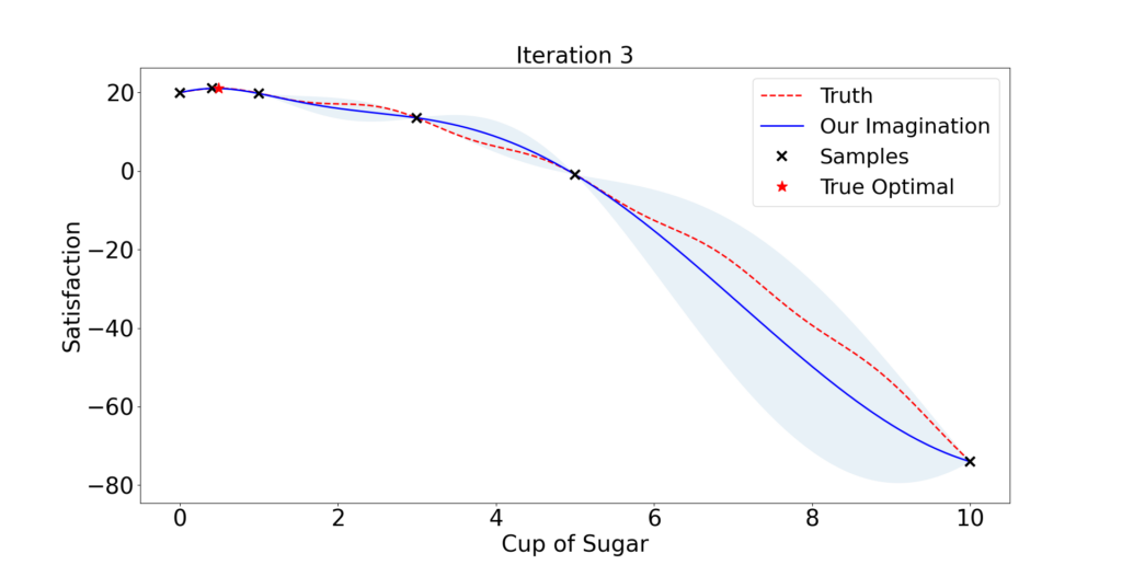
One plausible strategy is that we first have a basic understanding of the client’s preference after providing him with 3 cakes with various amounts of sugar: x = 1, 3, and 5.
Then we tactically select the amount of sugar the client might prefer and collect the feedback. We expect our understanding gets better and better following this process.
So what is a tactical selection?
It is an ad hoc opinion rather than rigorous mathematics. Given an initial understanding/model (blue curve in Figure 1.1), it is natural to use the best knowledge we have so far and select the maximizer of the blue curve x = 0.8.
If we are willing to take more risk, we possibly would also look into any place between x = 5 to 10, since no trials have been done in that region and anything could happen. A fair recommendation takes a balance between exploitation and exploration.
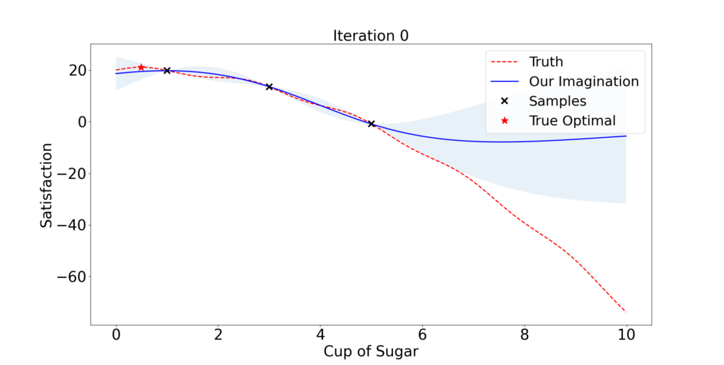
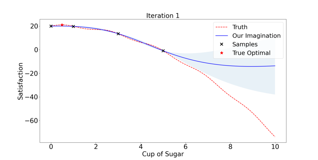
Following this principle, the algorithm finds out a near-optimal dose in only 2 iterations! But then he decides to take some risk and try x = 10. Quickly he finds out this client does not like too much sugar and probably stops there.
2. Gaussian Process Regression
Gaussian process regression is a statistical approach for modeling functions. It provides a Bayesian posterior that describes potential values for f_0(x) at a candidate point x.
Each time we observe f_0 at a new point and this posterior is updated. We offer a brief introduction here. A more complete treatment may be found in Rasmussen (2003).
Suppose the input pairs are (x_1, y_1),…,(x_T, y_T). We assume the observed data are generated from an unknown signal f plus a random noise

Furthermore, f’s values at x_1,…,x_T are assumed to be a sample from a multivariate Gaussian prior:

where the covariance matrix K is a T by T matrix whose (i, j)th entry equals k(x_i,x_j) for some kernel function k. Usually, K depends on a hyperparameter theta.
Example 1. (Kernel) A widely used Gaussian kernel k has the form:
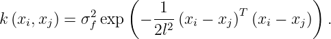
Here the hyperparameter is

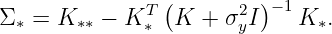
The ultimate goal is to make predictions f_* at new inputs X_* by figuring out the posterior distribution. We assume f and f_* are jointly normal:
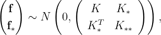
where K_*=k(X,X_*) and K_**=k(X_*,X_*).
One advantage of using Gaussian prior is that we will have closed-form posteriors regardless of what kernel we use.
Fact 2. The posterior distribution is Gaussian:

where
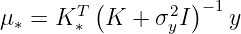
and
2.1 Update Prior Distribution
In each iteration, after we select and evaluate a new input, we want to update our understanding of the environment by choosing appropriate hyperparameters.
Typically the prior hyperparameter theta is estimated by a method called maximum likelihood estimation, which eventually ends up solving a non-convex problem

The above objective function is twice differentiable in theta. Hence, many global optimization algorithms, such as the quasi-Newton method L-BFGS-B, can be considered.
3. Propose sampling points
Having surveyed Gaussian processes, we return to the BO algorithm and discuss the so-called acquisition function that decides where the algorithm to sample next. Here, two well-known acquisition functions will be described, namely expected improvement and Gaussian process-upper confidence bound.
3.1 Expected Improvement
Expected improvement is defined as

where f(x+) is the value of the best sample so far and
We can obtain a closed form for the EI, with phi the probability density function of the standard normal distribution, Phi its cumulative function:

where

and mu, sigma is the posterior mean and standard deviation at x. Parameter xi determines the amount of exploration during optimization: Higher xi values lead to more exploration.
3.2 Gaussian Process-Upper Confidence Bound
Gaussian Process – Upper Confidence Bound (GP-UCB) picks x_{t} at round t by solving a problem:
where mu_{t-1} and sigma_{t-1} is the posterior mean and standard deviation conditioned on the observations (x_1,y_1),…,(x_{t-1},y_{t-1}); beta_t is a hyperparameter.
This objective function negotiates the exploration-exploitation tradeoff: It prefers both points x where f is uncertain (large sigma_{t-1}) and such where we expect to achieve high rewards (small mu_{t-1}).
4. Toy Example
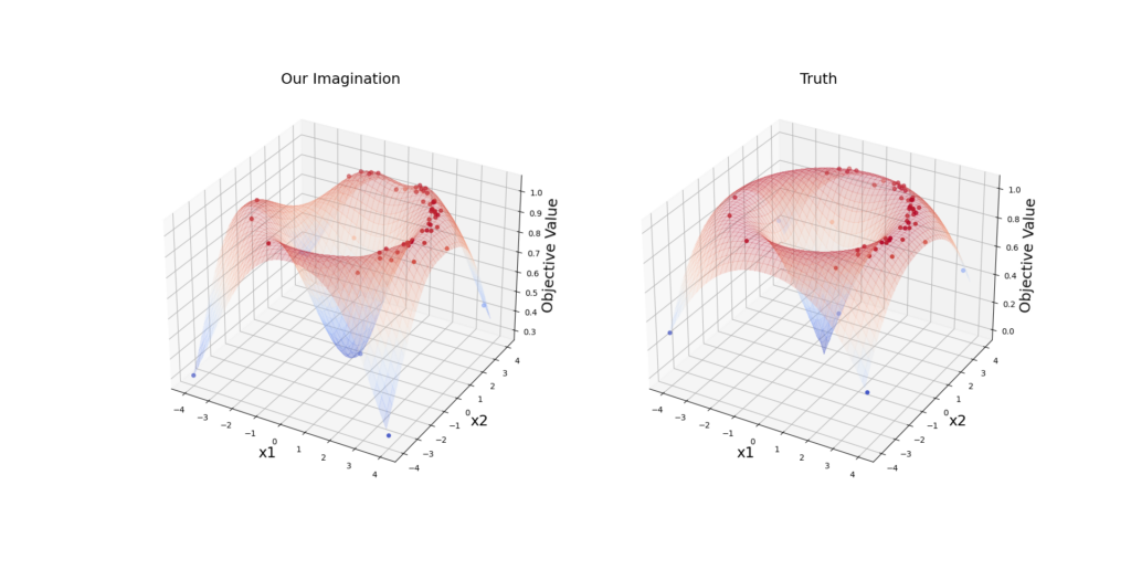
Now let us consider a sine maximization problem in a 2-dimensional space with Gaussian environmental noise N(0,0.01^{2}):
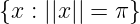
With some calculations, we figure out that in a noise-free environment, the maximizers locate on the surface of a sphere
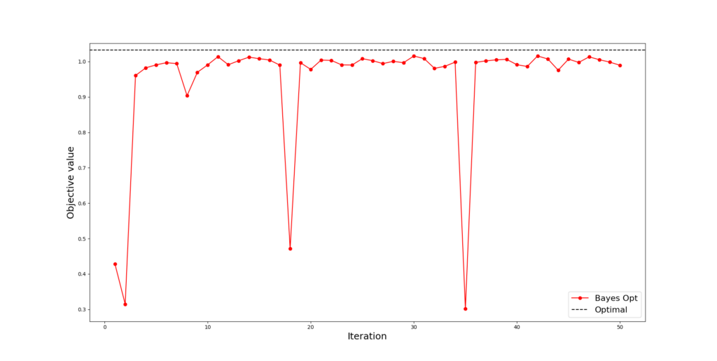
We started with 10 initial samples and in each round, we added a query point using the GP-UCB acquisition function.
In Figure 4.1, BO gets a near-optimal point after 12 rounds. When BO bravely explores the unknown regions, sometimes he can get very negative feedback (two downward peaks) but he promptly realizes that the optimal points can not be there and returns back to safe areas. In Figure 4.2, we observe that the model gets very close to the truth with only 50 iterations.
References
Rasmussen, C. E. (2003). Gaussian processes in machine learning. In Summer school on machine learning, pp. 6371. Springer.
