In Part 1, we discussed simple Bayesian optimization (BO), and now we further exam BO by taking into account uncontrollable contextual information and constraints.
Like in Part 1, our goal is still to maximize an unknown function. But in each round, we receive an additional context z_t in Z about the environmental conditions, e.g., outside air temperature, and have to choose an action s_t in S. If the observations are truly generated by a process depending on this context:

then we expect incorporating this side information will improve the performance.
Recall that BO consists of two components: prior updating and sampling points recommendation. Nothing will really change in the prior updating, except that now we are estimating the prior hyperparameters in an enlarged space S * Z, instead of S. For more details on this topic, see Krause and Ong (2011).
The main changes occur at the sampling points recommendation. Let us take Gaussian Process – Upper Confidence Bound (GP-UCB) as our acquisition function. Contextual Gaussian process upper confidence bound (CGP-UCB) algorithm naturally generalizes GP-UCB described in Part 1, which incorporates contextual information

where mu_{t-1} and sigma_{t-1} is the posterior mean and standard deviation of the GP over the joint set X=S * Z conditioned on the observations (s_1,z_1,y_1),…,(s_{t-1},z_{t-1},y_{t-1}).
When presented with context z_t, this algorithm uses posterior inference to predict mean and variance for each possible decision s, conditioned on all past observations (involving both the chosen actions, the observed contexts as well as the noisy payoffs).
Consider the following toy example: If the context z is positive, we want to maximize the action s; otherwise, we maximize -s:

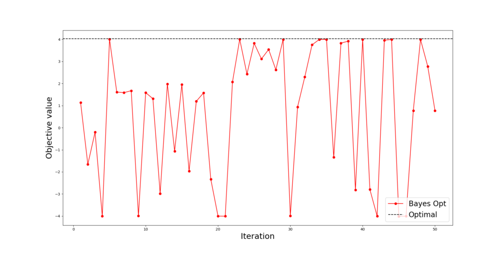
We started with 1 initial sample and in each round, we received a context uniformly drawn from [-4,4].
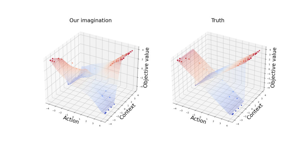
We observe that BO gets a near-optimal point after 5 rounds (Figure 1.1) and the model gets close to the truth with only 50 iterations (Figure 1.2).


Now we extend BO to the inequality-constrained optimization setting, particularly the setting in which checking a point satisfying all the constraints is just as expensive as evaluating the objective. More complete treatments can be found in Gardner et al. (2014) and Gelbart et al. (2014).
To understand the motivation of this topic, let us first go back to our cake-making example in Part 1: We want to maximize the client’s satisfaction, meanwhile, make sure that the cake contains no more than 200 calories.
The core idea we learned in BO: When something is unknown or expensive to evaluate, we bravely make a guess of its generating process and gradually update our belief when there is more evidence. Hence, we decide to place prior distributions on the constraint functions as well.
We start with problems that only have one constraint. For a known threshold lambda, the problem has the form


where both f_0 and g are expensive to evaluate.
Again, the change occurs at the sampling points recommendation. For a fixed training set, when we query a point, we solve


By introducing an indicator function, we are able to write the above problem into an unconstrained optimization. Let us write the feasible set C = {x: g(x) <= lambda} and define the indicator function as:

Then the constrained problem can be rewritten into an unconstrained one:

We are not done yet, since the objective function above still depends on the constraint function g, which is expensive to evaluate. So we place a prior on g.
During Bayesian optimization, after we have picked a candidate x_hat, we evaluate f_0(x_hat) and add (x_hat, f_0(x_hat)) to the set T_0 and we also now evaluate g(x_hat) and add ( x_hat , g(x_hat)) to the set T_g, which is then used to update the Gaussian process posterior

Assume the objective function f_0 and the constraint g are conditionally independent given an x. Then we end up with a weighted acquisition function:

where the randomness comes from different training sets.
Consider a constrained optimization in a 2-dimensional space:


First, let us have some preliminary analysis. When there is no inequality constraint, we will have the optimal points lie on a circle S_*={ x: ||x|| = pi/4} and the optimal value is sqrt(2).
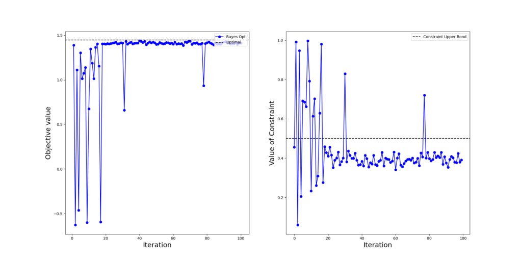
Let x_* be a member in the optimal set S_*. Now lambda=0.5 which is greater than sin( ||x_*||/2 ) = 0.38. Therefore, the optimal points of the unconstrained problem also satisfy the inequality constraint and we can attain the optimal value sqrt(2) of the unconstrained problem.
In Figure 2.1, we observe that the constrained BO gets a near-optimal feasible point after 20 rounds.

Gardner, J. R., M. J. Kusner, Z. E. Xu, K. Q. Weinberger, and J. P. Cunningham (2014).
Bayesian optimization with inequality constraints. In ICML, Volume 2014, pp. 937945. Gelbart, M. A., J. Snoek, and R. P. Adams (2014).
Bayesian optimization with unknown constraints. arXiv preprint arXiv:1403.5607. Krause, A. and C. S. Ong (2011).
Contextual Gaussian process bandit optimization. In Nips, pp. 24472455.